Annual Economic Report 2022
At its Annual General Meeting on Sunday 26 June 2022, the BIS released its Annual Economic Report and its Annual Report.
https://www.bis.org/publ/arpdf/ar2022e.htm
I. Old
challenges, new shocks-Viejos retos, nuevos choques -
https://www.bis.org/publ/arpdf/ar2022e1.htm
II. Inflation: a look under the hood
https://www.bis.org/publ/arpdf/ar2022e2.htm
III. The future monetary system
A burst of creative innovation is under way in money and payments, opening up vistas of a future digital monetary system that adapts continuously to serve the public interest
https://www.bis.org/publ/arpdf/ar2022e3.htm
I. Old challenges, new shocks
- Dos poderosas fuerzas -la pandemia del Covid-19 y la invasión rusa de Ucrania- determinaron los resultados económicos del pasado año.
- El crecimiento fue resistente, al menos hasta el estallido del conflicto entre Rusia y Ucrania. La inflación alcanzó máximos de varias décadas en un contexto de demanda intensiva de bienes y oferta limitada.
- Los riesgos de estanflación son grandes, debido a la alta inflación, la guerra en Ucrania y la ralentización del crecimiento en China. Las vulnerabilidades macrofinancieras preexistentes magnifican los riesgos, que podrían perturbar los sistemas financieros y tensar las economías de mercado emergentes.
- La tarea más apremiante de la política monetaria es restablecer una inflación baja y estable, limitando en lo posible el coste para la actividad económica y preservando la estabilidad financiera. A medio plazo, es necesario reconstruir de forma sostenible las reservas monetarias y fiscales. Los gobiernos deben volver a impulsar el crecimiento por el lado de la oferta
Durante gran parte del año, el crecimiento fue resistente. La economía mundial se expandió con fuerza en 2021, aunque en Estados Unidos y China no alcanzó las expectativas. A medida que avanzaba el año de revisión, la expansión perdió algo de impulso, con las limitaciones de la oferta, Omicron y la guerra de Ucrania como vientos en contra.
En este contexto, la inflación mundial subió a máximos de varias décadas. Al principio, el aumento de la inflación se consideró transitorio, ya que reflejaba el aumento de los precios relativos de un pequeño número de artículos afectados por la pandemia. Pero resultó ser persistente, ampliándose con el tiempo. En respuesta, los bancos centrales adelantaron en general el calendario y el ritmo del endurecimiento de las políticas. El aumento de la inflación y los cambios en las expectativas de la respuesta política provocaron episodios de volatilidad en los mercados financieros, y las condiciones financieras se endurecieron sustancialmente a medida que avanzaba el año, aunque partiendo de un estado excepcionalmente fácil.
Esta combinación de fuerzas hace que las perspectivas sean difíciles. La combinación de inflación elevada, precios altos y volátiles de las materias primas e importantes tensiones geopolíticas guarda un incómodo parecido con episodios pasados de estanflación mundial. Unas perspectivas de crecimiento inciertas en China refuerzan los riesgos a la baja. A diferencia del pasado, la estanflación actual se produciría junto con una mayor vulnerabilidad financiera, que incluye precios de los activos muy elevados y altos niveles de deuda, lo que podría magnificar cualquier desaceleración del crecimiento.
En este entorno, los responsables políticos se enfrentan a varios retos. A corto plazo, la prioridad es reducir la inflación, limitando en lo posible el coste para la actividad económica y preservando la estabilidad financiera1 . La reciente evolución económica complica aún más esta tarea. La política fiscal, en particular, se enfrenta a la presión de tener que hacer frente a la subida del coste de la vida y, en algunos países, aumentar el gasto militar, al tiempo que tiene que cumplir los compromisos a largo plazo de "ecologizar" la economía. Estos retos hacen que las reformas del lado de la oferta sean más importantes para promover el crecimiento sostenible.
Este capítulo describe en primer lugar los principales acontecimientos económicos y financieros del último año. A continuación, examina los riesgos de estanflación que se avecinan. Por último, se explican los retos políticos.
The year in retrospect
Global growth loses momentum as inflation returns
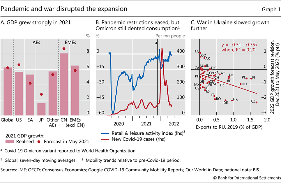
El año en cuestión comenzó bien. Se estima que el PIB mundial ha crecido un 6,3% en 2021, su tasa más rápida en casi 50 años, y en línea con las expectativas en el momento del Informe Económico Anual del año pasado (Gráfico 1.A).La expansión en 2021 tuvo una base amplia. Aparte de Japón, la mayoría de las economías avanzadas (EA) crecieron con fuerza, reforzadas por la relajación de la mayoría de las restricciones relacionadas con la pandemia y por una política fiscal y monetaria muy acomodaticia. El crecimiento de las economías de mercado emergentes (EME) (excluyendo a China) varió, pero en conjunto crecieron un 6,5%, apoyadas por el dinamismo del comercio mundial de bienes, la facilidad de las condiciones financieras mundiales y, en el caso de los exportadores de materias primas, la mejora de la relación de intercambio.
La evolución de China fue menos positiva. Es cierto que el PIB creció un sólido 8,1% en 2021. Sin embargo, no se cumplieron las expectativas. Las intervenciones reguladoras en los sectores inmobiliario y de las tecnologías de la información pesaron sobre la actividad. Además, los cierres más frecuentes y más amplios, en línea con la política de las autoridades de "cero-Covid dinámico", perturbaron las redes de suministro y socavaron el consumo.
La expansión mundial perdió impulso a medida que avanzaba el periodo de revisión. El aumento de las infecciones tras la aparición de Omicron a finales de 2021 redujo el gasto de los consumidores y, en algunos países, la oferta de trabajo (gráfico 1.B). Y, justo cuando la expansión se reanudó, la guerra en Ucrania supuso un nuevo golpe. Las previsiones de crecimiento del PIB para 2022 se redujeron, especialmente en los países más afectados por el conflicto (gráfico 1.C).
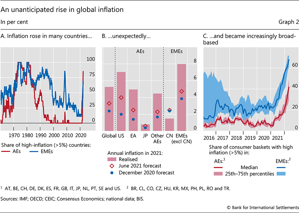
En una llamativa ruptura con el pasado reciente, la inflación mundial subió a máximos de varias décadas. A principios de 2022, superaba los objetivos de los bancos centrales en casi todas las EA, y había superado el 5% en más de tres cuartas partes de ellas (Gráfico 2.A). La proporción de EME con una inflación superior al 5% era casi igual de elevada. La inflación más alta fue menos frecuente en Asia. Pero incluso allí, en general, aumentó por encima del objetivo a medida que avanzaba el año, con la notable excepción de China.
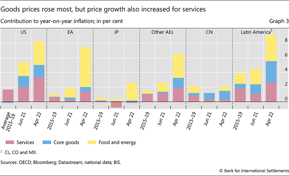
El repunte de la inflación fue una sorpresa para la mayoría de los observadores. A finales de 2020, las previsiones de inflación se situaban en general en los objetivos de los bancos centrales o por debajo de ellos (gráfico 2.B). Incluso a mediados de 2021, cuando la inflación ya había empezado a aumentar, la mayoría de los pronósticos subestimaron la magnitud o la persistencia del aumento2 . Estos aumentos de precios se interpretaron en general como ajustes de precios relativos puntuales o transitorios a los cambios de la oferta y la demanda inducidos por la pandemia. Pero la inflación se fue ampliando progresivamente (gráfico 2.C). A principios de 2022, el crecimiento de los precios de los servicios, que suele ser más persistente, superó su nivel anterior a la pandemia en gran parte del mundo (Gráfico 3).
Graph 3
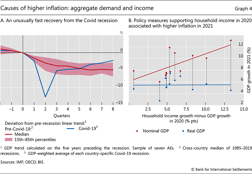
En primer lugar, la recuperación de la recesión de Covid ha sido inusualmente rápida, especialmente en las EA (Gráfico 4.A). El apoyo masivo de la política fiscal y monetaria al principio de la pandemia reforzó los ingresos de los hogares a pesar de las grandes caídas del PIB. Este aumento de los ingresos - gran parte del cual se ahorró inicialmente - allanó el camino para que el gasto se recuperara a medida que las restricciones de la actividad se relajaban en 2021. Sin embargo, parte de este gasto adicional se tradujo en un aumento de la inflación, de modo que la relación entre el apoyo a los ingresos al principio de la pandemia y la actividad económica en 2021 fue mucho más evidente para el PIB nominal que para la producción real (Gráfico 4.B).3 Mientras tanto, las medidas políticas, como los planes de suspensión de pagos y las moratorias de la deuda, ayudaron a evitar la temida ola de quiebras de empresas.4
Graph 4
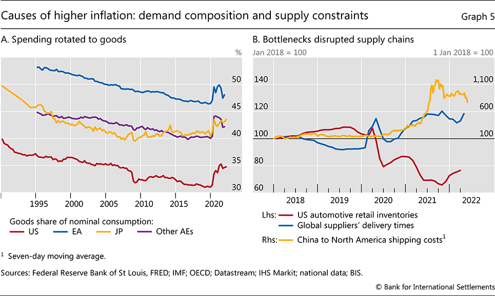
Second, the pandemic-induced rotation of aggregate demand to goods from services, especially contact-intensive ones, proved surprisingly persistent. Little demand rotated back, even after most containment measures were lifted (Graph 5.A). Strong price increases by firms operating at full capacity in industries facing high demand were not matched by slower price growth elsewhere.5 As a result, inflation rose even as output remained below its pre-pandemic trend and labour markets pointed to spare capacity.
Third, supply failed to keep up with surging demand. In particular, global value chains came under pressure.6 In some cases, the pressure reflected disruptions due to natural disasters, geopolitical conflicts and lockdowns; in others, simply the strength of demand. Thus, bottlenecks emerged in a number of areas, including container shipping and semiconductors, leading to sharp price increases (Graph 5.B).7 Since many bottlenecks affected goods and services located "upstream", ie near the start of production networks, the supply constraints had large spillovers across industries and countries. This caused long delivery delays and left many retailers short of inventory.
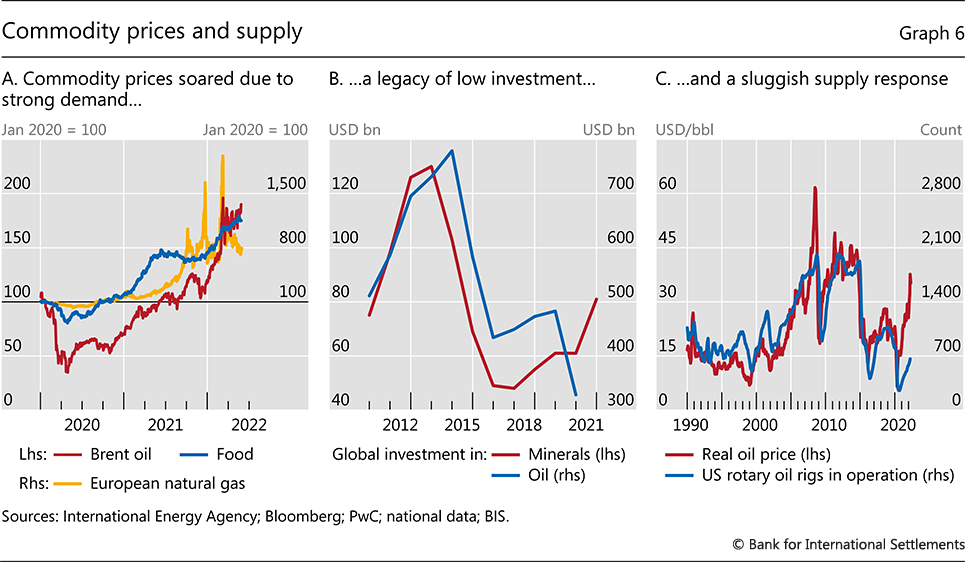
Supply was especially tight in energy and other commodity markets, triggering major price increases and higher volatility (Graph 6.A, Box A). In this case, a legacy of low investment by resource producers further restricted supply (Graph 6.B). Partly as a result, the supply response of marginal producers, such as those of shale oil, fell short of previous ones, which had helped to moderate commodity price shifts in the 2010s (Graph 6.C). The war in Ukraine further disrupted the global supply of products such as wheat, oil, gas, nickel, palladium and fertilisers.
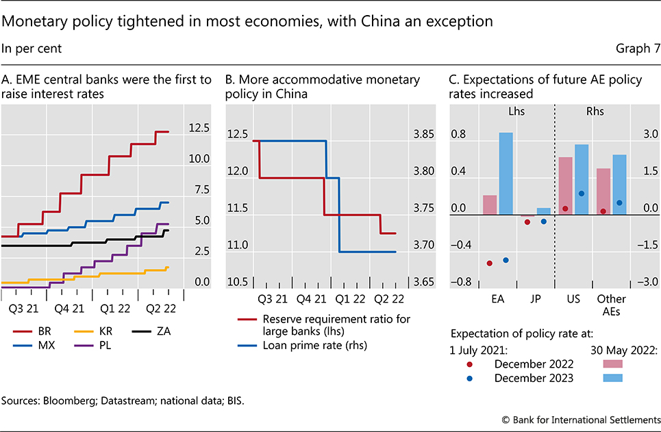
In several EMEs, central banks responded quickly to rising inflation. In Latin America, many had already raised policy rates several times by the end of 2021 (Graph 7.A). In Asia, where inflation was generally lower, policy tightening occurred later and more gradually. Still, by early 2022 most EME central banks had started to remove accommodation. The People's Bank of China was an important exception: it eased as the economy softened and inflation remained subdued (Graph 7.B).
Box A
Rising commodity prices: are we set for a repeat of the 1970s?
The past year has seen a significant rise in global inflation alongside higher commodity prices. This combination recalls the experience of the 1970s, particularly the aftermath of oil crises in 1973 and 1979. Those crises contributed to higher inflation and to a slowdown in global growth, which declined from an average of 5.5% in the decade leading up to the 1973 oil crisis to 2.5% in the following one. There are several reasons to expect recent commodity price rises to be less disruptive than those of the 1970s: recent price rises are proportionally smaller, albeit spread across a broader range of commodities, commodity supply has so far held up better, the global economy has become vastly more efficient in its use of many commodities, and the inflationary backdrop is more benign. That said, adverse outcomes are still possible if policymakers repeat the mistakes of the 1970s.
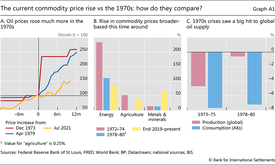
Recent commodity market developments differ from those of the 1970s
in several respects. The 1970s crises were concentrated in the oil
market. In the 1973 crisis, oil prices more than doubled in the space of
a month (Graph A1.A).
Prices rose to a similar extent in the 1979 crisis, albeit more
gradually. Recent oil price increases have been modest in comparison.
Oil prices have increased by around 50% since the middle of 2021,
although they briefly rose more after the start of the war in Ukraine in
late February. Taking a longer-term perspective, oil prices today are still within the
range of long-term averages, being at roughly the same level in nominal
(US dollar) terms as they were in mid-2014, and about 20% lower in real
terms. In contrast, the 1970s crises took oil prices to historic highs.
Taking a longer-term perspective, oil prices today are still within the
range of long-term averages, being at roughly the same level in nominal
(US dollar) terms as they were in mid-2014, and about 20% lower in real
terms. In contrast, the 1970s crises took oil prices to historic highs.
But while oil prices have so far increased by less than during the 1970s crises, a broader range of commodities has experienced price increases. The prices of non-oil energy, some agricultural goods, fertilisers and metals have all risen significantly over the past year, to be well above their pre-pandemic levels (Graph A1.B). Increases in European natural gas prices, which rose almost fourfold between the middle of 2021 and early 2022 and eight times from pre-pandemic levels, were particularly notable. In contrast, the 1970s crises were more concentrated in oil and, in the 1973 case, agricultural products.
Commodity supply disruptions have played a smaller role in recent
price increases than in the 1970s. Global oil production dropped by
around 5% around the 1973 oil crisis (Graph A1.C).
The decline in oil consumption in AEs was even larger, at around 8%,
due in part to embargos. Global oil production fell by less around the
1979 crisis, although oil consumption in AEs again decreased
substantially. In contrast, the rise in commodity prices over the past
year has been accompanied by a modest rise in the production of many
commodities, although not oil. That said, supply disruptions could
intensify over the coming year. The war in Ukraine will lower global
production of agricultural commodities such as wheat and maize, as well
as fertilisers. Meanwhile, sanctions on Russian oil and gas would represent an
effective reduction in the supply of these products, where Russia
accounted for around 12% and 17%, respectively, of global production in
recent years.
Meanwhile, sanctions on Russian oil and gas would represent an
effective reduction in the supply of these products, where Russia
accounted for around 12% and 17%, respectively, of global production in
recent years.
Aparte de las diferencias en el comportamiento de los mercados de materias primas, hay varias razones para pensar que el episodio actual podría desarrollarse de forma diferente a los de la década de 1970. El aumento de los precios de la energía, en particular, podría ser menos importante para el crecimiento hoy que en el pasado. La intensidad energética del PIB - la cantidad de energía necesaria para producir una determinada cantidad de bienes y servicios - ha caído en torno a un 40% desde finales de la década de 1970 (gráfico A2.A). La reducción ha sido más llamativa en el caso del petróleo, cuyo consumo se ha reducido a más de la mitad en relación con el PIB. Sin duda, parte de este hecho refleja un cambio en el uso de la energía del petróleo a otros combustibles, como el gas, cuyos precios también han subido recientemente. Pero incluso en el caso del gas, el consumo total por unidad de PIB es menor ahora que a finales de la década de 1970.
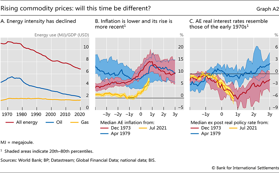
Las consecuencias de las recientes subidas de los precios de los productos básicos dependerán de la respuesta de los responsables políticos. Una razón para esperar resultados más favorables es que los marcos de política monetaria son muy diferentes. La crisis de 1973 siguió de cerca el colapso del régimen de tipos de cambio gestionados de Bretton Woods. En aquella época, los objetivos e incluso los instrumentos de la política monetaria estaban mal definidos en muchos países. Hoy en día, los bancos centrales disponen de marcos institucionales mucho más claros y sólidos. Aun así, la trayectoria de los tipos de interés reales durante el último año, al menos en las EA, guarda un sorprendente parecido con la de los años 70, con grandes descensos de los tipos de interés reales en el periodo previo a la crisis de los precios del petróleo en ambos episodios (Gráfico A2.C). Por el contrario, en la crisis de 1979 los tipos de interés reales se mantuvieron más estables ante la subida de los precios del petróleo y acabaron aumentando sustancialmente cuando los bancos centrales trataron de controlar la inflación.
La conducción de la política fiscal también es importante. En las EA, muchos gobiernos trataron de amortiguar el golpe a los ingresos de la crisis del petróleo de 1973 con medidas fiscales expansivas.icon el consiguiente aumento de la demanda agregada se sumó a las presiones inflacionistas. En cambio, las respuestas fiscales a la crisis del petróleo de 1979 fueron en general menos expansivas. El telón de fondo de la crisis actual es bastante diferente, ya que se prevé que los déficits presupuestarios se contraigan en la mayoría de las jurisdicciones a medida que los gobiernos retiren los estímulos desplegados en el momento álgido de la pandemia de Covid-19. Dicho esto, varios gobiernos han anunciado recortes fiscales o han ampliado las subvenciones en respuesta a las recientes subidas de los precios de los productos básicos, como ocurrió tras la crisis del petróleo de 1973.
icon Aunque el aumento de los precios del petróleo desde su mínimo en abril de 2020 ha sido mucho mayor, esos niveles bajos se produjeron tras un descenso de precios sin precedentes en las primeras fases de la pandemia. icon Véase Organización de las Naciones Unidas para la Agricultura y la Alimentación (2022). icon Véase Reis (2021). icon Véase Black (1985) y Roubini y Sachs (1989).
En las EA, los bancos centrales respondieron más lentamente. Al principio, muchos intentaron "mirar a través" de una inflación aparentemente transitoria más alta. Sin embargo, a medida que avanzaba el año de revisión, los bancos centrales redujeron su orientación hacia el futuro, señalando un inicio más temprano de la normalización de las políticas (Gráfico 7.C). En Estados Unidos, la Reserva Federal se inclinó en diciembre por un ritmo de endurecimiento más rápido y elevó el tipo de interés de los fondos federales en 75 puntos básicos al final del periodo de referencia. Varios bancos centrales de pequeñas economías abiertas también subieron los tipos de interés en varias ocasiones a principios de 2022. En la zona del euro, los participantes en el mercado adelantaron sus expectativas sobre el calendario de subidas de los tipos de interés, mientras que el BCE ajustó gradualmente sus orientaciones para aumentar la posibilidad de un endurecimiento más temprano de la política. El Banco de Japón siguió siendo una excepción, manteniendo su postura altamente acomodaticia.
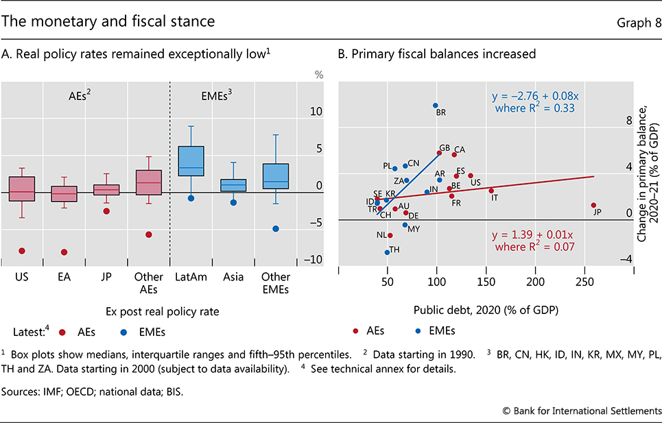
Nominal policy rates generally increased by less than near-term inflation. As a result, real ex post policy rates – ie adjusted for realised inflation – actually fell in most countries, from levels that were already exceptionally low. In most AEs, at the time of writing, real rates are 1–6 percentage points below their historical range over the past three decades (Graph 8.A). Real policy rates have generally been somewhat higher in EMEs, but remain negative in most.
Fiscal deficits declined in most countries. Improving economic conditions allowed governments to wind back some of the fiscal stimulus deployed at the height of the pandemic. In EMEs, fiscal constraints loomed large and countries with higher debt levels generally implemented larger fiscal consolidations (Graph 8.B). While fiscal deficits generally shrank in AEs, governments in the United States and Europe laid the groundwork for large infrastructure programmes in the coming years.
Inflation and war shape financial conditions
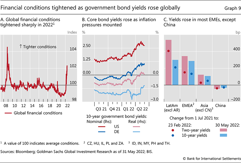
Higher inflation and the outbreak of war in Ukraine also left an imprint on financial markets. Financial conditions tightened sharply during the review period, particularly from the start of 2022, as asset prices responded to the prospect of rising inflation and the resulting anticipated monetary policy tightening (Graph 9.A). The extent of the tightening varied across countries and asset classes, reflecting their different exposures to economic and geopolitical developments.
The consequences of the shifting macroeconomic conditions were first evident in sovereign bonds. In the core bond markets, nominal yields rose sharply in October 2021, particularly at shorter maturities. Long-term yields followed from December as the Federal Reserve flagged an earlier and faster policy tightening, before moving sharply higher after the start of the war in Ukraine (Graph 9.B). The rise in US yields initially reflected higher inflation compensation, particularly at shorter maturities. But real long-term yields also increased materially after the start of the war. Indeed, in May the yield on 10-year Treasury Inflation-Protected Securities became positive for the first time since the start of the pandemic (light red line). In the euro area, German real yields remained deeply in negative territory (light blue line), despite a jump in May as the ECB flagged an earlier rise in policy rates. Over the entire period, however, the rise in German yields was due largely to increased inflation compensation.
Shifts in the shape of the US yield curve amid faster than anticipated monetary tightening raised concerns about the economic outlook. Starting in October, the US yield curve flattened as short-term yields rose by more than long-term ones. In March, it briefly inverted, which is often seen as a signal of an imminent recession. In the event, the inversion was short-lived and reversed sharply in early April. Such a flattening was not observed in the euro area and Japan, reflecting their slower pace of monetary tightening.
In EMEs, sovereign yields also increased alongside inflation. Initially, they rose more in Latin America, where inflationary pressures were strongest and many central banks had already started tightening policy early in 2021 (Graph 9.C). The increase of sovereign yields in eastern Europe accelerated after the outbreak of war in Ukraine, reflecting these countries' greater exposures to the conflict. Asian economies generally saw smaller sovereign yield increases, as inflation was slower to gain momentum in the region. In China, yields declined, as policymakers wrestled with the fallout of a troubled real estate sector and renewed Covid outbreaks.
Tighter US financial conditions spilled over globally through an appreciation of the US dollar. The appreciation proceeded in two steps. The first, lasting from late 2021 to March 2022, was gradual, reflecting evolving inflationary concerns and expectations that monetary tightening would proceed more quickly in the United States than in other AEs (Graph 10.A). EME exchange rate movements were more varied. Commodity exporters, particularly in Latin America, even saw their exchange rates appreciate on the back of widening interest rate differentials and rising commodity prices (Graph 10.B). The renminbi also strengthened gradually, supported by a large current account surplus and portfolio inflows.
Graph 10
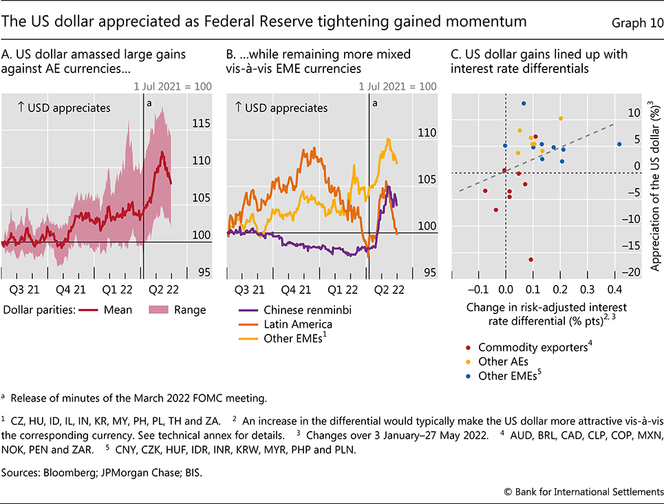
From April, the pace of US dollar appreciation increased sharply, before retracing somewhat in late May. The appreciation coincided with the large upward shift in the US yield curve, the reversal with renewed concerns about the global growth outlook. Overall, since the beginning of 2022 the US dollar appreciated most against the currencies of non-commodity exporters that were less advanced in their tightening cycles, as reflected in the expected changes in risk-adjusted interest rate differentials (Graph 10.C). Also in the second quarter, gold prices gave up the modest gains amassed earlier in the year, while cryptocurrencies, particularly ethereum and bitcoin, plummeted to their lowest levels since mid-2021. Some stablecoins, such as tether, deviated significantly from their benchmarks, while others broke down completely in a manner resembling the collapse of traditional exchange rate pegs.8 Capital outflows from most EMEs, however, were moderate, signalling the surprising resilience of investor sentiment towards this asset class in the face of tighter global financial conditions.
Corporate credit conditions tightened significantly as the year progressed. Relative to their distribution since the Great Financial Crisis (GFC), investment grade credit spreads saw the sharpest increases, although spreads in all rating categories rose from historical lows to levels exceeding their post-GFC medians (Graph 11.A). The relatively muted rise in high-yield credit spreads was partly due to rising investor demand for floating rate debt – more prevalent in the high-yield segment – at a time of higher expected future policy rates. It may also have reflected falling liquidity in high-yield corporate debt markets, particularly in the euro area, which delayed the full repricing of riskier debt.
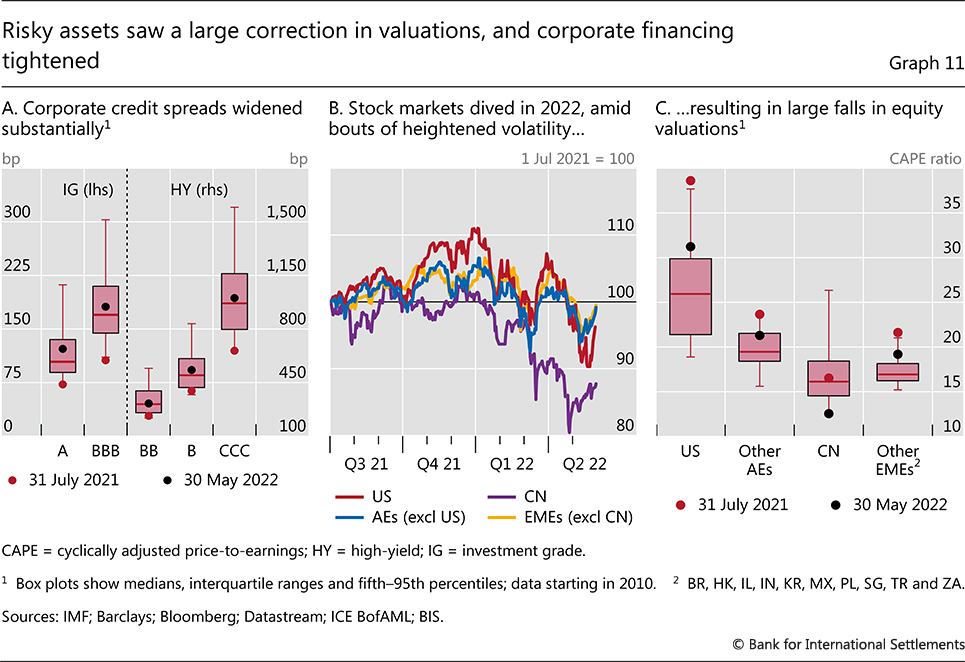
Equity markets saw large fluctuations amid broad sectoral divergences. Stock prices generally rose in the first half of the review period, albeit with bouts of volatility as higher inflation and Omicron rattled investor sentiment (Graph 11.B). They then fell significantly in 2022 in the wake of the Federal Reserve's tightening shift and the expectation that other central banks would follow suit, as well as the outbreak of the war. In most regions, valuations declined, although they generally remained above their post-GFC medians (Graph 11.C).
Chinese equities were an important exception. They drifted down from early 2022, as problems in the real estate sector lingered and Covid-related lockdowns intensified (Graph 11.B). The rout accelerated after the beginning of the war, with Chinese assets – both stocks and bonds – seeing large outflows, leaving valuations at post-GFC troughs (Graph 11.C).
Stagflation: how high are the risks?
Aunque el crecimiento mundial fue en general resistente durante el periodo de revisión, los riesgos a la baja son grandes. En gran medida, esto refleja la naturaleza única de la recesión de Covid y la posterior expansión, que ha provocado mayores presiones inflacionistas junto con elevadas vulnerabilidades financieras, especialmente el alto endeudamiento en un contexto de aumento de los precios de la vivienda. Esta combinación no tiene precedentes históricos. Antes de mediados de la década de 1980, las recesiones solían ir precedidas de una elevada inflación y del consiguiente endurecimiento monetario, mientras que el sistema financiero estaba muy reprimido. Desde entonces, aparte de Covid, las recesiones han seguido normalmente a los picos del ciclo financiero, y la inflación ha permanecido moderada durante las expansiones y, por tanto, ha exigido relativamente poco endurecimiento de la política monetaria.La ausencia de paralelos históricos hace que las perspectivas sean muy inciertas. Como mínimo, será necesario un período de crecimiento inferior a la tendencia para que la inflación vuelva a niveles aceptables. Pero una modesta desaceleración podría no ser suficiente. La reducción de la inflación podría implicar importantes costes de producción, como tras la "Gran Inflación" de los años 70. Incluso entonces, la inflación podría no caer rápidamente, dada la intensidad de las recientes presiones sobre los precios. En el peor de los casos, la economía mundial podría verse abocada a un periodo de estanflación, que implicaría tanto un bajo crecimiento, si no una recesión total, como una alta inflación.
¿Cómo podría producirse esta situación de estanflación? El afianzamiento de los recientes resultados inflacionistas elevados, reforzados por el aumento de los precios de las materias primas, sería un punto de partida natural. Los altos precios de las materias primas también podrían pesar sobre el crecimiento mundial, al igual que una desaceleración significativa de la economía china. Las tensiones financieras podrían magnificar la desaceleración del crecimiento. Las EME están especialmente expuestas.
A new inflation era?
Los regímenes de inflación tienen propiedades de autorrefuerzo (capítulo II). Al igual que la baja inflación contribuyó a moderar el aumento de los salarios y los precios antes de la pandemia, los recientes resultados de la alta inflación pueden dar lugar a cambios de comportamiento que podrían afianzarla. Este cambio es más probable si un aumento de la inflación es lo suficientemente grande y persistente - es decir, destacado - para dejar una gran huella en la vida de los trabajadores y las empresas, y si éstos tienen suficiente poder de negociación y de fijación de precios para desencadenar una espiral de precios y salarios.Hay varios indicios de que los recientes aumentos de la inflación han sido destacados. Por ejemplo, las búsquedas en Internet sobre el precio de la gasolina se dispararon a principios de marzo (gráfico 12.A). Y las medidas de las expectativas de inflación, tanto de los hogares como de los participantes en los mercados financieros, han empezado a aumentar (Gráfico 12.B).
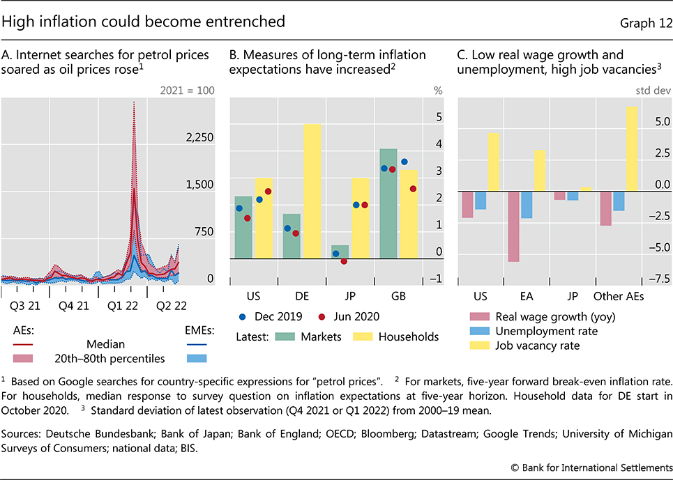
At the same time, the conditions for faster wage and price growth look to be in place. Real wages grew unusually slowly over the past year, and declined in some jurisdictions, even as labour market conditions were remarkably tight, with job vacancy rates well above their historical averages and unemployment rates low (Graph 12.C). In part, this reflects the fact that wages tend to be negotiated infrequently, and so naturally take time to respond when inflation increases unexpectedly. As existing wage agreements expire, workers are likely to seek larger wage rises. In some countries they have already secured wage indexation clauses to guard against future inflation surprises.9 Meanwhile, the recent broadening of inflation pressures suggests that many firms have greater pricing power than they had pre-pandemic.
La guerra en Ucrania
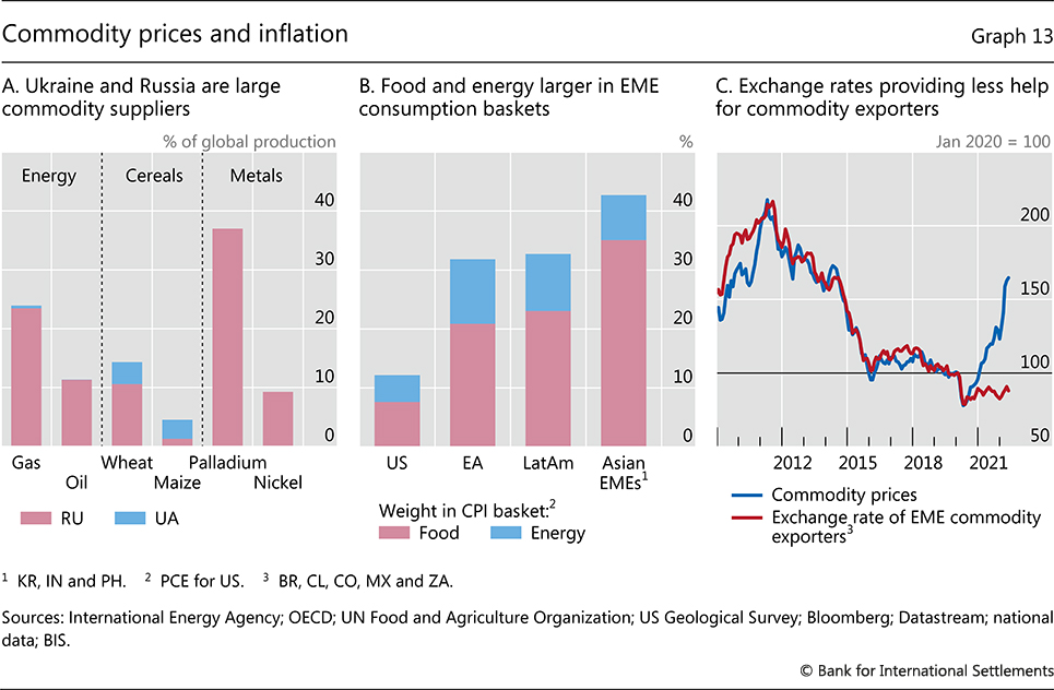
La guerra en Ucrania se suma a las presiones inflacionistas. El principal canal es el aumento de los precios de los productos básicos, en particular del petróleo, el gas, los productos agrícolas y los fertilizantes, de los que Rusia y Ucrania son importantes productores (gráfico 13.A). Algunas de estas subidas de precios -por ejemplo, las del petróleo y el trigo- repercutirán directamente en la inflación. Las EME se verán más afectadas que las EA, dada la mayor proporción de alimentos y energía en las cestas de consumo (Gráfico 13.B). Las apreciaciones de los tipos de cambio pueden reducir las presiones sobre los precios de las importaciones en las EME exportadoras de productos básicos, aunque esta relación parece haberse debilitado desde el inicio de la pandemia (Gráfico 13.C). Otras subidas de precios, por ejemplo de los metales, elevarán los costes de producción de las empresas y podrían intensificar las presiones sobre los precios a través de las cadenas de valor mundiales.
The net effect of these factors could be material, particularly as inflation is already high. Estimates of the effect of commodity price increases across a broad panel of countries indicate that a 30% increase in oil prices, combined with a 10% rise in agricultural prices – roughly in line with those seen since the start of the year – has historically been associated with a 1 percentage point increase in inflation in the following year (Graph 14.A).10 For European countries, where gas prices have surged even more than oil prices, the effects could be larger.
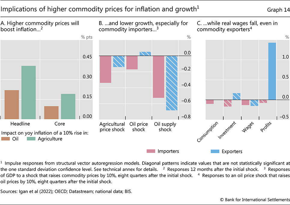
Commodity market disruptions will also weigh on growth (Graph 14.B). By raising firms' production costs, higher commodity prices effectively lower global aggregate supply. Although commodity exporters will benefit from higher export revenues, largely in the form of higher corporate profits, the growth boost could be smaller than usual if tighter financial conditions and expectations that the rise in commodity prices will be temporary deter firms from investing to boost capacity (Graph 14.C).11, 12 Meanwhile, for commodity importers, the terms-of-trade loss will further compress domestic incomes and aggregate demand. The hit to growth could be even larger if higher commodity prices are accompanied by a cut to global commodity output and rationing, as occurred in the 1970s.
This speaks to possible broader consequences of the war, beyond its effect on commodity markets. Admittedly, the hit to trade flows is relatively small on a global scale. But the conflict has created an environment of higher uncertainty and political risk, which is historically associated with lower business investment.13 And over the longer term, the new geopolitical landscape could see real and financial fragmentation, including through a reorganisation of global supply chains.
Slower growth in China
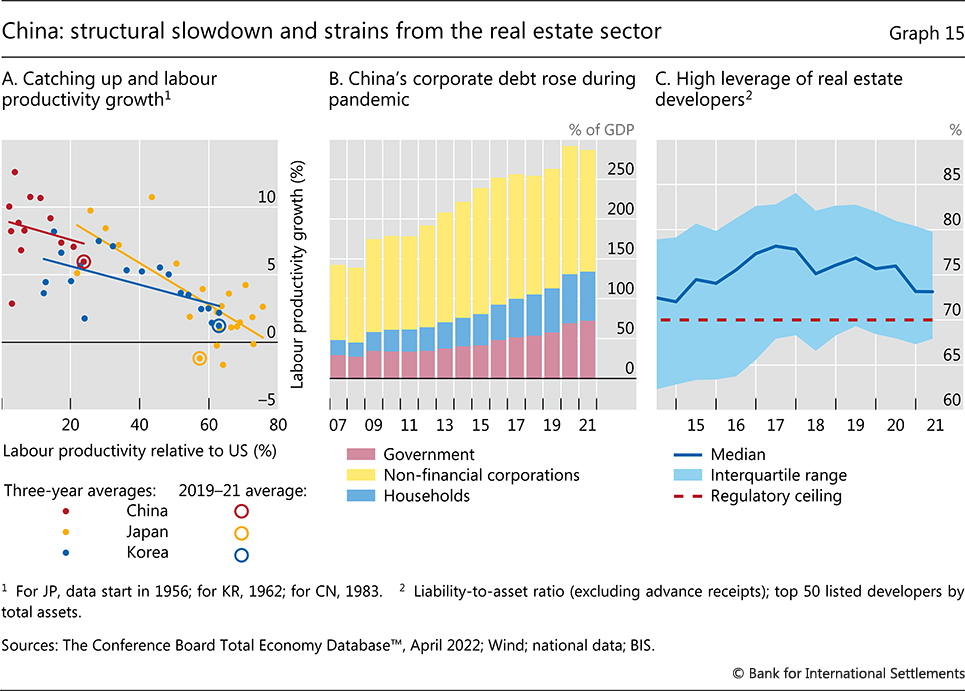
La evolución de China podría ser una nueva fuente de presión estanflacionaria mundial. Por un lado, el país ha representado una parte considerable del crecimiento mundial - alrededor de una cuarta parte - durante las dos últimas décadas. Además, ha sido una importante fuente de demanda externa para el resto del mundo, sobre todo de materias primas. Por otra parte, la entrada de China en el sistema comercial mundial ejerció persistentes presiones desinflacionistas, especialmente en las economías avanzadas, incluso cuando su demanda interna hizo subir los precios de las materias primas14 .Algunos de los factores que contribuyen a la ralentización del crecimiento de China son estructurales y, por tanto, es probable que sean duraderos. La población china en edad de trabajar, que alcanzó su punto máximo a principios de la década de 2010, seguirá disminuyendo en los próximos años. Entretanto, el potencial de aumento de la productividad derivado de la incorporación de tecnología preexistente y de la reasignación de mano de obra a actividades de mayor productividad ha disminuido. La ralentización del crecimiento de la productividad del trabajo a medida que China se ha ido acercando a la frontera tecnológica es comparable, en líneas generales, a la de Japón y Corea en décadas anteriores (Gráfico 15.A). Esto sugiere que es poco probable que se vuelvan a alcanzar tasas de crecimiento de la productividad muy elevadas.
Un descenso prolongado del ciclo financiero supondría un nuevo lastre para el crecimiento. En un contexto de elevados niveles de deuda, la influencia de los factores financieros ya era evidente en el año examinado. En respuesta a la nueva acumulación de deuda corporativa durante la pandemia, y al continuo y elevado apalancamiento de los promotores inmobiliarios, las autoridades chinas introdujeron varias medidas para reducir las vulnerabilidades inmobiliarias en la segunda mitad de 2021 (Gráfico 15.B y C). Estas medidas redujeron la capacidad de endeudamiento de los promotores, lo que llevó a algunos a retrasar los pagos de la deuda y a desprenderse de activos, y redujeron los préstamos hipotecarios a los hogares. Estas medidas mejoran la sostenibilidad del crecimiento a largo plazo, pero frenan el crecimiento a corto plazo (Recuadro B). De hecho, la relajación de algunas medidas a principios de 2022 pone de manifiesto el difícil equilibrio de las autoridades.
Los acontecimientos relacionados con la pandemia agravan los vientos en contra a corto plazo. Los cierres locales y otras medidas para hacer cumplir la estricta política de Covid podrían perturbar aún más las redes de producción, tanto dentro de China como con los socios comerciales.15 La lucha contra el virus está lejos de terminar.
Macro-financial vulnerabilities
China no es ni mucho menos el único país con importantes vulnerabilidades macrofinancieras. Más de una década de condiciones financieras excepcionalmente acomodaticias, reforzadas por la respuesta política a la pandemia, ha dejado a las empresas y a los hogares de muchos países altamente endeudados y ha contribuido a elevar los precios de los activos, especialmente los inmobiliarios. Inusualmente, estas vulnerabilidades no disminuyeron materialmente durante la recesión de Covid. De hecho, en la mayoría de los países los niveles de endeudamiento privado, sobre todo del sector empresarial no financiero, aumentaron sustancialmente (Gráfico 16.A).
The coexistence of elevated financial vulnerabilities and high inflation globally makes the current conjuncture unique for the post-World War II era. The tighter monetary conditions needed to bring down inflation could cast doubt on assets – including housing – priced for perfection on the assumption of persistently low real interest rates and ample central bank liquidity. Even traditionally more secure assets could be exposed. Bonds, for example, have provided a safe haven for investors in the low-inflation environment of recent decades. During this phase, bad economic times, when the prices of riskier assets like equities typically fall, were generally met with monetary easing, which boosted bond prices (Graph 16.B). But when inflation is high, economic downturns are more likely to be triggered by tighter monetary conditions, causing both bond and stock prices to fall.
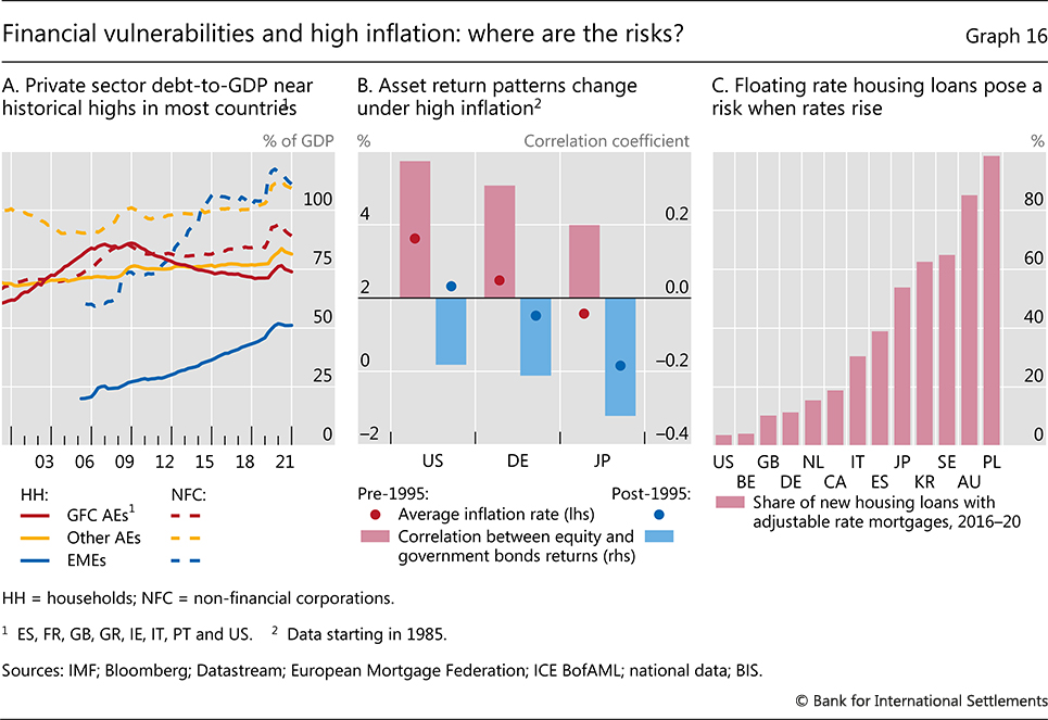
The effects of tighter monetary conditions would also be felt through higher debt repayments. The largest strains are likely in countries where floating rate loans – sensitive to higher policy rates – are more common (Graph 16.C). In this regard, several small open economies look particularly exposed, at least in their household sectors. For firms, floating rate loans are more common among riskier segments. In principle, the aggregate savings built up early in the pandemic could provide buffers for households and firms to cope with higher rates, at least initially. However, the incidence of higher savings may not match that of debt burdens.
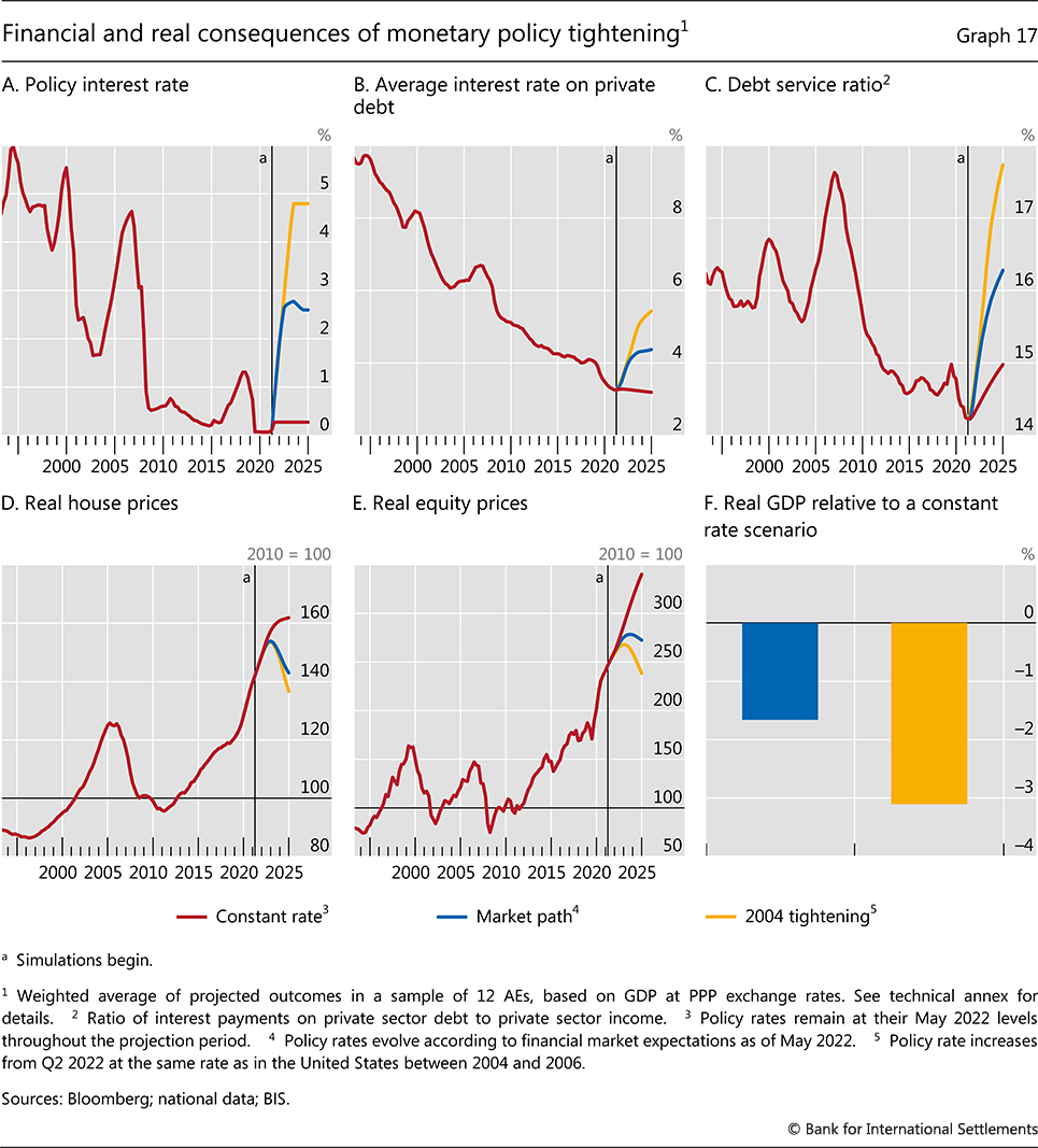
The consequences of these vulnerabilities for economic activity will depend on how high interest rates rise and how asset prices and debt servicing burdens respond. Illustrative simulations based on historical relationships between financial and economic variables can shed light on the key risks. Particularly in countries where a large portion of debt is at fixed rates, it will take some time for the interest rates faced by households and firms to reflect higher policy rates (Graph 17.A and 17.B). Despite these lags, average AE private sector debt service ratios (DSRs) could rise by more than 1 percentage point by 2025, to their highest level in over a decade, if central bank policy rates evolve as financial markets currently expect (Graph 17.C). If rates were to mirror the larger 425 basis point increase in the federal funds rate in the 2004–06 period, average DSRs could increase by more than 2 percentage points, reaching their pre-GFC peak.
Box B
The real estate sector's evolving contribution to China's growth
El análisis utiliza datos del mercado de la vivienda a nivel de provincia y los relaciona con el PIB a nivel de país.icon Dado que las condiciones económicas locales ejercen una gran influencia en la actividad del sector de la vivienda, los indicadores a nivel de provincia pueden ayudar a identificar la evolución que los datos a nivel nacional ocultan. Además, desde un punto de vista metodológico, los datos a nivel de provincia proporcionan más variación en las variables que se analizan, lo que ayuda a precisar las relaciones económicas.icon
La relación entre el sector inmobiliario y el crecimiento del PIB de China se reforzó en la década de 2010. Mientras que las medidas de la actividad inmobiliaria a nivel de provincia, como las viviendas iniciadas, no muestran una relación significativa con el posterior crecimiento del PIB antes de 2010, después de este año aparece una relación significativa (Gráfico B1.B). Esto es coherente con la creciente proporción de la inversión residencial en la producción de China.
Los indicadores del sector inmobiliario también pueden ayudar a predecir el PIB. En particular, una medida de la sobreoferta de viviendas a nivel provincial -calculada como superficie iniciada menos superficie vendida- señala un menor crecimiento del PIB en un horizonte de dos años (Gráfico B1.C). Una relación similar, aunque de signo contrario, se da en el caso de las viviendas iniciadas y la actividad de inversión residencial en un horizonte de un año. Estas relaciones reflejan los efectos directos e indirectos de la inversión residencial sobre el PIB, por ejemplo, los efectos indirectos sobre otros sectores, como los servicios inmobiliarios, la producción de materiales de construcción y las ventas al por menor relacionadas con la mejora de la vivienda.
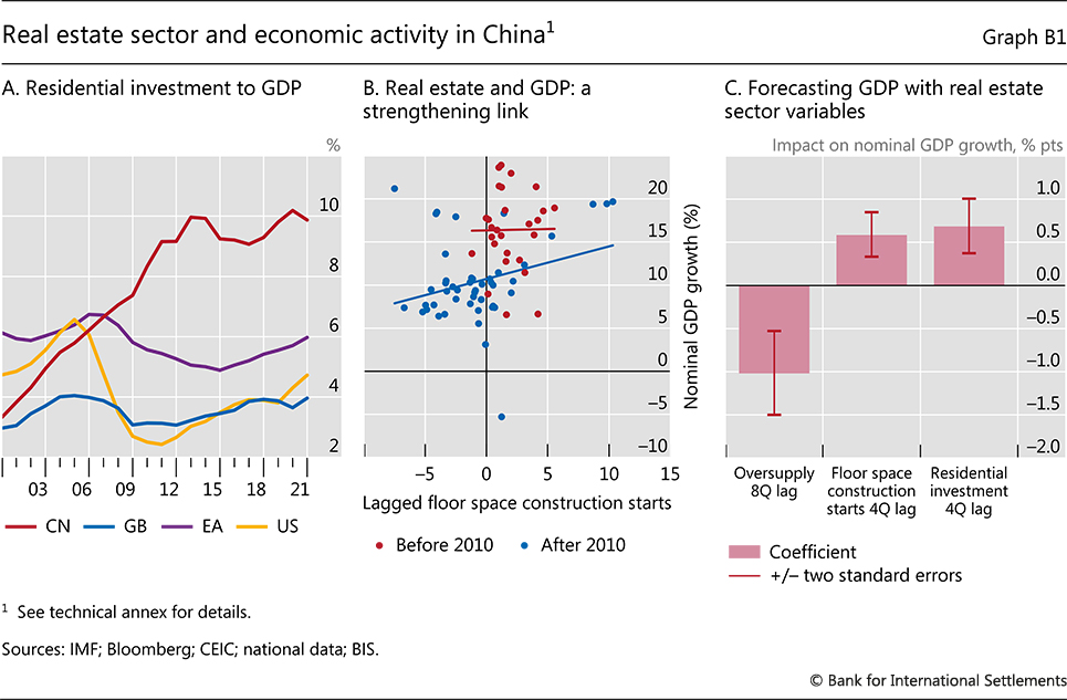
These results confirm that the slowdown in the housing sector is
likely to have had a material effect on China's growth over the past
year. To give a sense of the magnitudes, the estimates suggest that, if
growth in floor space starts and residential investment had stayed at
their average levels in 2018–19, and growth in housing oversupply at its
2018 level, real GDP growth (year-on-year) would have been some 1–1.5
percentage points higher in 2021. That said, such estimates are by their
nature uncertain, in part because they assume that the relationships
between the variables remain stable and that the causation runs
exclusively from the real estate indicators to GDP. Moreover, the model
does not explicitly control for financial factors or changes in housing
market policies, including macroprudential measures, which are also
likely to have contributed to China's housing market dynamics.
For analysis on China's housing boom, see Fang et al (2015) and Glaeser et al (2017). See Jordà et al (2016), Leamer (2015) and Kohlscheen et al (2020).  For detailed analysis, see Kerola and Mojon (2022).
  Indeed, aggregated province-level housing market indicators explain a
larger share of the variation in China's GDP growth than aggregate
country-level housing data; the opposite is true for exports and
imports, where country-wide measures prove more informative. This result
is obtained by aggregating information from province-level data by
principal component analysis and then comparing with nation-wide
indicators.
Indeed, aggregated province-level housing market indicators explain a
larger share of the variation in China's GDP growth than aggregate
country-level housing data; the opposite is true for exports and
imports, where country-wide measures prove more informative. This result
is obtained by aggregating information from province-level data by
principal component analysis and then comparing with nation-wide
indicators.  Accounting for sectoral linkages and spillovers by means of
input-output tables, Rogoff and Yang (2021) argue that the impact of the
real estate sector on China's GDP is close to 30%. In this comparison
as well, China's real estate sector appears larger than those in other
major economies. See Kuttner and Shim (2016).
Accounting for sectoral linkages and spillovers by means of
input-output tables, Rogoff and Yang (2021) argue that the impact of the
real estate sector on China's GDP is close to 30%. In this comparison
as well, China's real estate sector appears larger than those in other
major economies. See Kuttner and Shim (2016).
In this environment, asset prices could come under pressure. According to the simulations, the path of real house prices would resemble that around the GFC, while the long post-GFC run-up in equity prices would start to retreat (Graphs 17.D and 17.E). In contrast, if policy rates were to remain at their current levels, asset prices and debt levels would continue to rise, implying a further build-up in vulnerabilities.
Such shifts in DSRs and asset prices could have a material effect on economic activity. The simulations suggest that the level of GDP in the average AE would be about 1.5% lower under the market interest rate path than it would be if policy rates were held constant (Graph 17.F). In the steeper "2004 tightening" scenario, the level of GDP would be around 3% lower. Even these results may understate the GDP response to tighter monetary conditions, which would occur against a backdrop of historically high debt levels, whose effects on growth may be felt more keenly when asset prices are falling, and the growth headwinds of the higher commodity prices and enhanced geopolitical uncertainty described above.16
Naturally, the results of this simulation exercise are purely illustrative. In particular, they are based on average historical relationships since the mid-1980s, which may have evolved over the past four decades. The use of cross-country averages also masks considerable variation in exposure to higher policy rates across jurisdictions. And, even for individual countries, the simulations are subject to considerable uncertainty. Nonetheless, they help to highlight key vulnerabilities and give a sense of the orders of magnitude involved.
Financial system stress
Financial system disruptions could reinforce any slowdown in household and corporate spending. Such disruptions could come from stresses in banks or non-bank financial intermediaries (NBFIs). Consider the two sectors in turn.
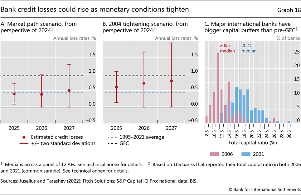
An economic downturn against the backdrop of high debt levels would test banks' resilience. Credit losses are most likely to accrue in the medium term, after rising policy rates have passed through into market rates and households and firms have exhausted accumulated buffers.
The size of credit losses will depend on the degree of required policy tightening. If macro-financial conditions follow the "market path" scenario shown in Graph 17 until the end of 2024, past relationships suggest that expected bank credit losses over 2025–27 would be close to historical norms across AEs, albeit with considerable uncertainty (Graph 18.A). They would be larger in the scenario where rates follow the "2004 tightening" scenario shown in Graph 17, somewhat closer to those experienced in the GFC (Graph 18.B). That said, stronger capital cushions mean that banks are in a much better position to take the hit than they were then (Graph 18.C).
Developments in NBFIs could pose greater challenges.
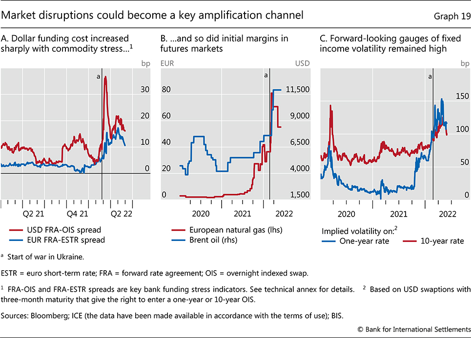
Financialised commodity markets are a key pressure point. These markets came under strain when the war in Ukraine broke out, as sharp rises in commodity price volatility triggered large margin calls in derivatives markets. The frantic search for cash to meet those calls briefly led to stress in dollar funding markets, as reflected in the spreads to OIS of forward rate agreement rates (Graph 19.A). At the same time, some futures markets saw substantial increases in initial margin requirements, leading some commodity traders to stop hedging their exposures in those markets and absorb price risk themselves (Graph 19.B). This, in turn, saw commodity end users, such as airlines, face difficulties hedging their own exposures. While the tensions ultimately eased, the underlying vulnerabilities could resurface if price volatility spikes again.
Some sovereign bond markets could also face strains as monetary conditions tighten. The unwinding of large central bank bond purchases will remove reserves from the banking system and could prove disorderly, as the ructions in US repo markets in September 2019 showed. Already, liquidity in US Treasury markets diminished in late 2021 as broadening inflationary pressures led investors to anticipate an imminent policy shift. Market conditions worsened further as the review period progressed, with implied volatilities in fixed income markets near historical peaks, particularly for short-term rates (Graph 19.C).
As well as market functioning, sovereign credit spreads could emerge as a concern as central banks wind down asset purchases. Some European government bond markets are a case in point, given very high debt levels and past experiences. As credit risk is repriced, these worries could also have a significant impact on financial institutions' balance sheets, probably affecting both securities dealers – key participants of the NBFI ecosystem – and banks, which hold substantial amounts of government bonds in their portfolios.
A broader concern is that the extent of exposures among NBFIs, which could transform stresses at individual institutions into more systemic disturbances, are not well known. The collapse of Archegos Capital Management in April 2021, and the attendant stock market disruptions, is a leading example. In that instance, not only was the capital of Archegos largely wiped out, but several banks that provided it with prime brokerage services also took significant hits to their own capital buffers. While the fallout was ultimately contained, it nonetheless highlights the risks posed by hidden leverage in loosely regulated corners of the financial system.
Emerging market economies
The risks discussed above pose tough tests for EMEs. This is despite improvements in fiscal and monetary policy frameworks that, together with greater use of prudential buffers and macroprudential tools, have made EMEs generally more resilient.
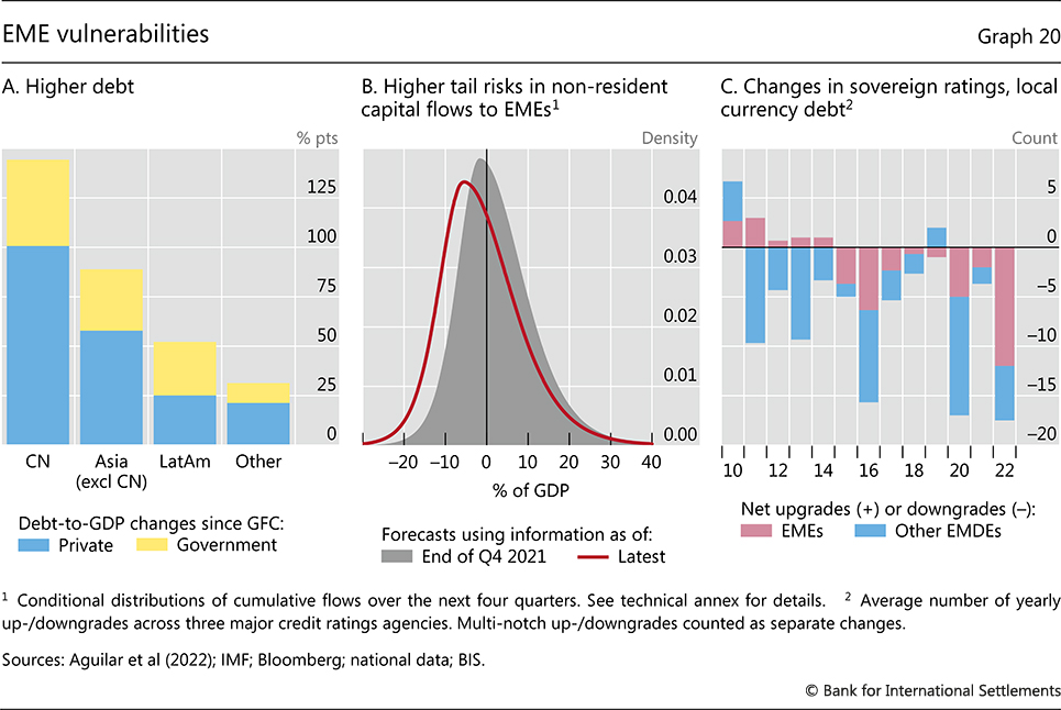
Challenges arise because, in some other respects, the starting point for EMEs is worse than in the past. Many are facing tighter financial conditions against a backdrop of high debt, which rose further during the pandemic (Graph 20.A). This raises the prospect of increased capital outflows, which have historically accompanied times of rising global interest rates.17 The rise in geopolitical tensions at the current juncture amplifies such risks (Graph 20.B). For commodity exporters, the rise in commodity prices counteracts outflow pressures. Nonetheless, a number of sovereigns have recently seen rating downgrades (Graph 20.C).
Many EMEs are highly exposed to stagflationary risks. Growth prospects had already deteriorated pre-pandemic, with potential growth rates on average 2 percentage points lower than before the GFC.18 In addition, in many EMEs pandemic scarring is more evident than in AEs. By the first quarter of 2022, the median length of full school closures due to Covid-19 had amounted to 29 weeks in Latin America and 16 weeks in emerging Asia, compared with six weeks in AEs.19 Labour force participation is also recovering more slowly. In Latin America, in particular, participation rates in 2021 were some 2 percentage points below pre-pandemic levels.20 Many EMEs are highly exposed to slower Chinese growth, especially countries in emerging Asia and some commodity exporters (Graph 21.A). And, in countries where vaccination rates lag, health and economic activity could be more vulnerable to further pandemic waves.
Even if growth does not decline, higher inflation tends to be more disruptive in EMEs. Since inflation expectations are less well anchored in some of these countries, not least in Latin America, larger nominal policy rate increases are required to control inflation. Surging food prices are also more disruptive. Sharp rises in food prices have been associated with social instability and the imposition of export controls in the past, with recent price levels surpassing those seen during the food price spike of 2011 (Graph 21.B).21 And while regulated food and energy prices, and the associated subsidies, will lower the immediate pass-through to headline inflation in some EMEs, they come with a fiscal cost and can create economic distortions.22 Combined with growing demands for social spending in the pandemic's aftermath, larger fiscal deficits could eventually feed through into exchange rate depreciations and inflation (Chapter II).
Macroeconomic policy challenges
Los recientes acontecimientos plantean una serie de retos de política macroeconómica. La elevada inflación es sin duda uno de los principales, complicado además por las frágiles perspectivas de crecimiento y las vulnerabilidades financieras. En este entorno, podría ser difícil lograr un aterrizaje suave, es decir, volver a situar la inflación en el objetivo de forma sostenible sin frenar bruscamente la expansión. Al mismo tiempo, la necesidad de reconstruir los colchones monetarios y fiscales a medio plazo, que es evidente desde hace tiempo, sigue siendo acuciante. El entorno actual crea una oportunidad para la normalización sostenida de la política monetaria, pero complica la tarea de la política fiscal. De hecho, para lograr la normalización de la política a medio plazo y mejorar los resultados macroeconómicos de forma más general, será necesario depender menos de la política de estabilización macroeconómica para sostener el crecimiento y dar un nuevo impulso al fortalecimiento de la capacidad productiva de la economía.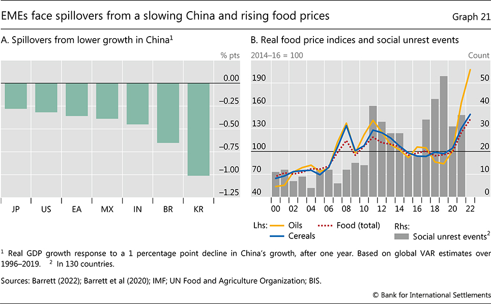
Controlling inflation
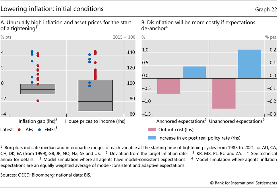
El reto más acuciante para los bancos centrales es restablecer una inflación baja y estable sin, a ser posible, infligir graves daños a la economía. Al menos en las EA, los bancos centrales no se han enfrentado a este reto durante décadas. Históricamente, lograr ese "aterrizaje suave" ha resultado difícil, y las condiciones de partida son en muchos aspectos desfavorables (Recuadro C). En la mayoría de los países, las tasas de inflación son mucho más altas de lo habitual al comienzo de un ciclo de endurecimiento, y los tipos de interés oficiales reales y nominales mucho más bajos, lo que sugiere que puede ser necesario un endurecimiento más fuerte para controlar la inflación (Gráfico 22.A). Al mismo tiempo, los elevados precios de los activos y los altos niveles de deuda significan que los costes de producción de unas condiciones financieras más estrictas podrían ser mayores que en el pasado.El destacado papel de las variaciones de los precios relativos en el impulso de la inflación complica la respuesta política. La receta estándar de los libros de texto es "mirar a través" de este tipo de inflación porque el endurecimiento necesario para evitarla sería costoso23 . A la luz de la experiencia reciente, es más difícil defender una distinción tan clara. Si los ajustes de los precios relativos son persistentes y el aumento de la inflación desencadena efectos de segunda ronda, los bancos centrales no tienen más remedio que responder.
Calibrar la respuesta implica naturalmente un compromiso. Endurecer demasiado y con demasiada rapidez podría infligir un daño innecesario. Pero hacer demasiado poco aumentaría la perspectiva de un endurecimiento mayor y más costoso en el futuro.
For much of the past two decades, central banks had exceptionally ample leeway to lean towards a more accommodative approach. In particular, inflation was generally at or below central bank targets, even where unemployment rates reached multi-decade lows. Of course, trade-offs did not disappear. A decade or more of historically low interest rates contributed to a build-up of financial vulnerabilities and meant that central banks did not rebuild monetary buffers.
Box C
How likely is a soft landing?
Most central banks are now starting to tighten policy, often in the face of high inflation. A key question is whether they will be able to engineer a "soft landing" – ie a tightening cycle that ends without a recession. This box examines what historical monetary policy tightening cycles can teach us about the likelihood of a soft landing and what factors are associated with it.
The first step is to identify policy tightening cycles and soft
landings. The analysis is based on tightening cycles in a panel of 35
countries over the period 1985–2018. A tightening episode is defined as
one in which the nominal monetary policy rate increases in at least
three consecutive quarters.
The tightening cycle ends when the policy rate peaks before a
subsequent decline. If an economy enters a recession, defined as two
consecutive quarters of negative GDP growth, in the three years after
the peak of the policy cycle, the landing is defined as a hard one. If
the economy avoids a recession, the landing was soft. Historically, about half of all monetary policy tightening cycles have ended in a soft landing, as defined above.
Tightening cycles that end in hard landings differ from those that
end in soft landings in several respects. A key one is that hard
landings are more likely when monetary tightening is preceded by a
build-up of financial vulnerabilities. In particular, faster growth in
credit relative to GDP prior to a tightening episode is associated with
hard landings (Table C1, top panel). Intuitively, financial
vulnerabilities are likely to reinforce the contractionary effects of
tighter monetary policy on GDP growth. Moreover, heightened
vulnerabilities mean that a growth slowdown is more likely to trigger a
recession. The influence of credit growth on the probability of a hard
landing is also consistent with the observation that financial cycle
peaks have tended to coincide with recessions since the early 1980s,
lining up with the sample in this exercise.
Financial vulnerabilities are more likely to emerge when interest
rates are low. Reflecting this, hard landings are also commonly
associated with low real interest rates prior to the start of the
tightening episode. For example, the average real policy rate at the
start of tightening cycles that end in hard landings is 0.4%, compared
with 1.4% at the start of those that end in soft landings. Inflation is
also on average higher before hard landings than it is before soft ones,
although the difference between the two is not statistically
significant.
The policy rate trajectory during a tightening episode can also influence the likelihood of a soft landing. In particular, hard landing episodes tend to involve increases in policy rates that play out over a longer time (middle panel of Table C1). However, neither the average speed of a policy tightening, nor the size of overall tightening, seems to be associated with differences in the likelihood of hard or soft landings. This suggests that there is little to be gained in terms of output from a shallower and more drawn-out tightening path.
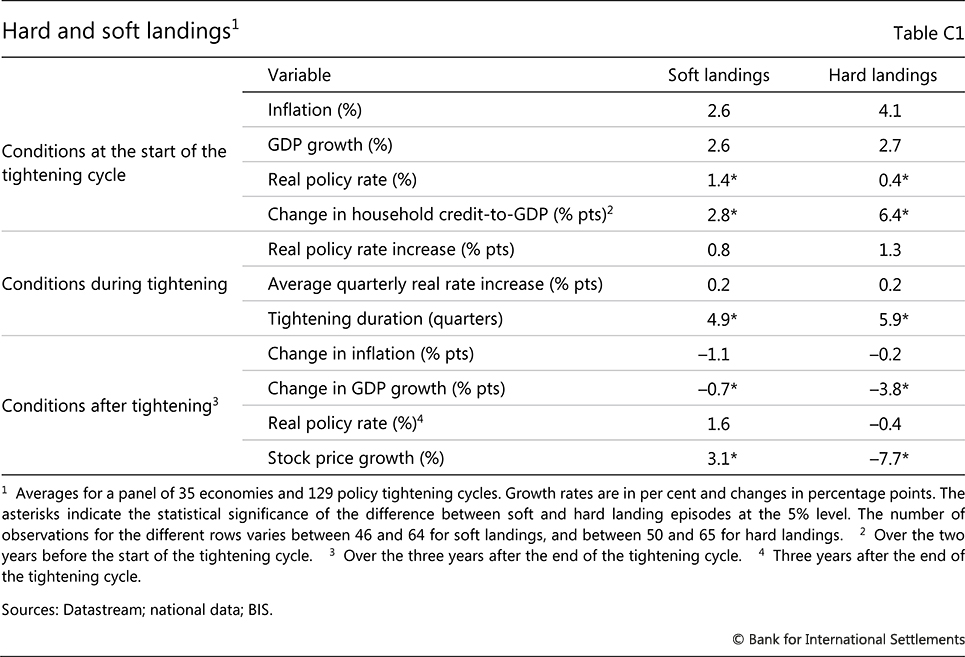
What are the consequences of a hard landing, beyond lower GDP growth? Hard landings are more likely to be associated with abrupt stock price falls (bottom panel of Table C1). At the same time, they are more likely to be followed by lower real interest rates, which often become negative. These findings suggest that achieving a soft landing could be key to ensuring a sustainable normalisation of monetary policy settings to allow buffers to be rebuilt over the medium term.
While the analysis above is silent about the underlying policy frameworks, there are a number of ways in which they could increase the likelihood of a soft landing. Some relevant dimensions have seen notable improvements in recent decades. For example, the greater use of macroprudential tools and larger financial system buffers could weaken the relationship between credit growth and hard landings, by increasing the resilience of the economy against shocks. Better anchoring of inflation expectations may reduce the required policy tightening in response to inflationary pressures, through its stabilising impact on wage and price-setting (Chapter II).
We do not consider the role of balance sheet, exchange rate or credit policies in policy tightening.
There is no standard definition of a hard landing. The results are
unchanged when one defines a hard landing based on the peak-to-trough
GDP growth following the end of the tightening cycle. The results are
also similar when a horizon of two rather than three years is considered
after the end of the tightening cycle. See Borio et al (2018).
Because most of the tightening cycles in the sample occurred after
central banks had adopted inflation targeting, or similarly credible
policy regimes, the results may understate the adverse effects of high
inflation and de-anchored inflation expectations on the likelihood of
experiencing a hard landing.
The new inflationary environment has changed the balance of risks. Gradually raising policy rates at a pace that falls short of inflation increases means falling real interest rates. This is hard to reconcile with the need to keep inflation risks in check. Given the extent of the inflationary pressure unleashed over the past year, real policy rates will need to increase significantly in order to moderate demand. Delaying the necessary adjustment heightens the likelihood that even larger and more costly future policy rate increases will be required, particularly if inflation becomes entrenched in household and firm behaviour and inflation expectations (Graph 22.B).
Policy normalisation
A second macroeconomic policy challenge is to deliver a durable policy normalisation. As discussed in last year's Annual Economic Report, this requires achieving macroeconomic objectives consistent with central bank mandates and room for policy manoeuvre. The pandemic and the war in Ukraine have highlighted the imperative to hold buffers so that macroeconomic policy can deal not only with inevitable, cyclical recessions, but also truly unanticipated events.
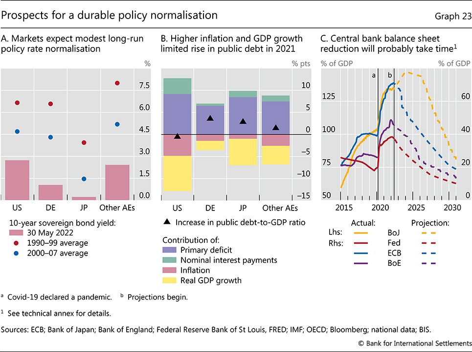
Such an outcome is by no means guaranteed. Even in countries where financial markets anticipate rapid monetary tightening, long-term bond yields still point to very low policy rates at the peak of the adjustment, often negative in real terms (Graph 23.A). Few fiscal authorities project a material decline in public debt in the years ahead, even though the constellation of real interest rates is substantially below real GDP growth rates, thereby greatly favouring a debt drawdown.24 Indeed, higher energy and food prices have been creating substantial pressure for more government spending to ease cost of living pressures.
Some governments have already stepped up spending, and further expenditures, often untargeted, loom on the horizon. Germany, the Philippines, Sweden and the United Kingdom, for example, have announced cash transfers to vulnerable households to alleviate cost of living increases, while France and Korea have temporarily lowered sales taxes on energy products.25 Brazil and Turkey have cut import tariffs on food. In Europe, proposed increases in defence expenditure could also have a material impact on public finances. Commitments to address climate change add further pressure on fiscal positions globally. And less visible fiscal commitments linked to ageing populations loom large.
A major difference from previous years is higher inflation. In the near term, this provides a pressing reason to normalise monetary policy. Moreover, the unexpected inflation burst will erode to some extent the value of long-term fixed income debt. Because it rose much faster than interest rates in 2021, higher inflation helped limit the rise in debt-to-GDP ratios (Graph 23.B). However, surprise inflation is not a mechanism that fiscal or monetary authorities can or should rely on to control public debt over the medium term. If it occurred repeatedly, unexpected inflation could make investors demand a sizeable risk premium. And higher interest rates will make fiscal policy normalisation harder.
The large stocks of government debt held by central banks complicate matters. As explained in last year's Annual Economic Report, they raise the sensitivity of overall fiscal positions to higher rates. In effect, they transform long-term fixed income debt into debt indexed at the overnight rate (the interest rate on bank reserves). The effect can be quite large. Where central banks have used such purchases more extensively, some 30–50% of public debt in the large AE jurisdictions is in effect overnight.26
The general picture brings into sharp focus the tensions between fiscal and monetary policy along the normalisation path. These could heighten the pressure on central banks to keep their stance more accommodative than appropriate and delay the already lengthy return of central bank balance sheets to more normal levels (Graph 23.C). This puts a premium on institutional arrangements that safeguard central bank independence and a clear emphasis on the primacy of low and stable inflation as the core monetary policy objective.
Central banks have some options to influence the likelihood of a successful policy normalisation. Choices about the pace and timing of policy tightening, as well as the sequencing of balance sheet adjustment and interest rate increases, could all influence the smoothness of the process. Effective communication is critical. Here, central banks face a trade-off between forward guidance and flexibility. Setting clear guidelines and benchmarks for policy normalisation could help steer financial markets and reduce disruptions as interest rates rise. But if forward guidance is interpreted as a degree of pre-commitment, it can curtail the central banks' flexibility to respond to evolving conditions. This flexibility is essential.
Rebooting the supply side
The experience of the past year, ranging from supply chain bottlenecks to conflict-induced stagflationary pressures, reinforces the importance of reigniting growth-friendly expenditure, in particular investment, and supply-side reforms. These could raise growth and make it more resilient, thus facilitating the normalisation of monetary and fiscal policies over time. To the extent that some of the measures will involve carefully targeted expenditure increases that provide benefits only further down the road, in an environment of limited fiscal space, there is also a premium on making the tax system more growth-friendly.
As one of the most urgent tasks, the green transition calls for targeted measures to put in place a more durable and sustainable energy mix. Simulations suggest that an orderly transition that features a timely increase in green energy investment could impose relatively small near-term costs and deliver persistent long-term gains, measured in terms of economic output (Graph 24.A). By contrast, a disorderly shift, where the adoption of clean energy technology lags but carbon-intensive energy sources are shut down rapidly, would involve significant costs in both the short and long run. The war in Ukraine has sharpened the focus on energy security, which, especially over the longer run, is consistent with the push to "green" the economy. That said, in the near term, energy security considerations are likely to delay the green transition in some countries by increasing the demand for coal and shale gas, for example. Moreover, the near-term transition costs could be higher than conventionally assumed and may create additional fiscal burdens.
Para aumentar el crecimiento sostenible, y cuando el espacio fiscal lo permita, muchos países podrían beneficiarse de un mayor gasto en capital humano y físico. Un gasto en educación mayor y mejor orientado ayudaría a compensar las pérdidas de escolarización y competencias durante la pandemia, especialmente en los países con niveles de renta más bajos. Antes de la pandemia, la duración media de la escolarización era unos cinco años más corta en los países emergentes de Asia (ocho años) que en las economías avanzadas (13 años); en América Latina, la diferencia con respecto a las economías avanzadas era de unos cuatro años27.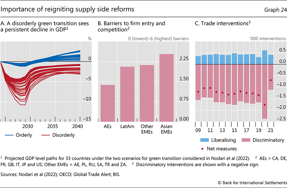
Otra prioridad es mantener unos mercados competitivos y abiertos y evitar la fragmentación real y financiera, especialmente ante las tensiones geopolíticas y el aumento de los precios de los alimentos. La reducción de las barreras a la entrada de empresas y a la competencia ayudaría a acomodar los cambios inducidos por la pandemia en las preferencias de los consumidores y a acercar a las empresas a la frontera de la productividad (gráfico 24.B). En los últimos años se han incrementado las medidas comerciales restrictivas, y los altos precios de los alimentos aumentan el riesgo de nuevas restricciones a la exportación (Gráfico 24.C). Tras la pandemia y en respuesta al aumento del riesgo geopolítico, es probable que las cadenas de suministro experimenten algunos ajustes, incluida la deslocalización, destinados en parte a aumentar su resistencia. Si bien algunos de estos ajustes son necesarios y deseables, será importante evitar los crecientes impulsos a favor del nacionalismo y la fragmentación, dada la importancia del comercio para el crecimiento y la productividad mundiales.
En términos más generales, la necesidad de reformas estructurales subraya que no se puede lograr un crecimiento mayor y duradero sólo mediante políticas de estabilización macroeconómica. El uso repetido y sistemático de dichas políticas durante la última década ante la debilidad económica, junto con las dificultades para reconstruir los colchones en épocas de bonanza, es una de las razones por las que el margen de maniobra de la política macroeconómica ha disminuido tanto con el tiempo. Se necesita urgentemente un cambio de rumbo.
Endnotes
1 See also Chapter II.
2 See Budianto et al (2021).
3 Because the increase in demand was particularly strong for internationally tradeable, durable goods, expansionary fiscal measures may also have had large international inflationary spillovers; see de Soyres et al (2022).
4 See Banerjee et al (2020) and Mojon et al (2021).
5 As shown in Graph 3, price growth in the services sector – which was more affected by pandemic-related restrictions – generally picked up in the year under review, albeit not to the same extent as goods prices.
6 See Santacreu and LaBelle (2022) and Shin (2021).
7 See Rees and Rungcharoenkitkul (2021).
8 See also Chapter III.
9 According to Hernández de Cos (2022), 30% of collective bargaining agreements in Spain in the first three months of 2022 linked final wage increases to inflation, up from 17% in 2021.
10 See Igan et al (2022) for estimates of the effects of commodity price movements on growth and inflation.
11 Particularly in some oil exporters, much of the revenue boost will accrue to state-owned enterprises rather than the private sector.
12 Rees (2013) and Kulish and Rees (2017) discuss the different investment implications of temporary and permanent commodity price shocks.
13 See Caldara and Iacoviello (2022).
14 For evidence on the contribution of imports from lower-wage countries to reduced price pressures in AEs, see eg Auer et al (2013).
15 For estimates regarding the costs of lockdowns in China that take account of trade linkages across cities, see Chen et al (2022).
16 Similarly, the research on "GDP at risk" documents that downside risks to growth increase when financial conditions are tighter; see Adrian et al (2019).
17 See Box I.F in BIS (2021).
18 Potential GDP growth is proxied by Consensus GDP growth forecasts for six to 10 years.
19 Based on UNESCO map on school closures (https://en.unesco.org/covid19/educationresponse) and UIS, March 2022 (http://data.uis.unesco.org).
20 Based on data from ILO database.
21 Commodity price increases have also, on occasion, been a source of social tension in AEs, with the "gilets jaunes" protests in France in 2018–19 being a prominent recent example.
22 For weights of administered and regulated prices in various EME inflation measures, see eg Table 3.1 in Patel and Villar (2016).
23 See Aoki (2001).
24 On average, government debt in AEs is projected to decline by just 3 percentage points of GDP, from around 116% of GDP to 113% of GDP, between 2022 and 2027. In EMEs, it is projected to increase by almost 10 percentage points, from 67% of GDP to 77% of GDP. See IMF (2022) and BIS (2021).
25 See IMF (2022).
26 See Borio and Disyatat (2021).
27 Based on data from the World Economic Forum Global Competitiveness Index.
28 See OECD (2021).
Technical annex
Graph 1.A: Country groups calculated as weighted averages using GDP and PPP exchange rates. "Other AEs" is based on data for AU, CA, CH, GB and SE. "EMEs excl CN" is based on data for AR, BR, CL, CO, HU, ID, IL, IN, KR, MX, MY, PE, PH, RU, SA, SG, TH, TR and ZA.
Graph 2.B: December 2021 year-on-year inflation. Country groups calculated as weighted averages using GDP and PPP exchange rates. "Other AEs" is based on data for AU, CA, CH, GB and SE. "EMEs (excl CN)" is based on data for BR, CL, CO, HK, ID, IN, KR, MX, MY, PE, PL, RU, SA, SG, TH, TR and ZA.
Graph 3: "Other AEs" is an average of AU, CA, CH, DK, GB, NO, NZ and SE, weighted by GDP and PPP exchange rates. "Latin America" is a simple average of CL, CO and MX. "Food and energy" includes alcoholic beverages.
Graph 4.A: Based on data for AU, CA, EA, GB, JP, SE and US.
Graph 4.B: Based on data for AU, BE, CA, DE, ES, FR, GB, IT, NL, PL, SE and US.
Graph 5.A: "Other AEs" is an average of AU, CA, DK, GB, NO, NZ and SE, weighted by GDP and PPP exchange rates.
Graph 5.B: Suppliers' delivery times PMIs are displayed on an inverted scale. Shipping costs correspond to the Freightos Baltic daily containerised freight rate index.
Graph 6.C: Real oil price calculated as WTI crude oil price deflated by US CPI.
Graph 7.C: Based on one-month AUD, CAD, CHF, EUR, GBP, JPY, SEK and USD overnight index swap forward rates. "Other AEs" calculated as the simple average of AUD, CAD, CHF, GBP and SEK.
Graph 8.A: Ex post real policy rate defined as the difference between the policy rate and the year-on-year inflation rate. Country groups calculated as simple averages. "Other AEs" is based on data for AU, CA, CH, GB and SE. For CH, EA, KR, ID and TH, latest data refer to May 2022; for AU, to March 2022; for the remaining countries, to April 2022.
Graph 9.A: Goldman Sachs Financial Conditions index (FCI), which is a weighted average of country-specific riskless interest rates, exchange rate, equity valuations and credit spreads, with weights that correspond to the estimated impact of each variable on GDP.
Graph 9.C: Country groups calculated as simple averages.
Graph 10.A: Based on US dollar exchange rates for AUD, CAD, CHF, EUR, GBP, JPY, NOK, NZD and SEK.
Graph 10.B: Country group indices calculated as simple averages. "Latin America" is based on data for BR, CL, CO, MX and PE.
Graph 10.C: The risk-adjusted interest rate differential corresponds to the carry-to-risk ratio. This is calculated as the 12-month US dollar interest rate spread over corresponding country rates in their respective local currencies, as implied by forward and spot exchange rates, divided by the option-implied volatility of the exchange rate. "Other AEs" based on US dollar exchange rates for CHF, DKK, EUR, GBP, JPY, NOK and SEK.
Graph 11.A: Each rating bucket is constructed from GDP and PPP exchange rate-weighted averages of euro area and US ICE BofA ML corporate spread indices.
Graph 11.B: Country groups calculated as weighted averages using GDP and PPP exchange rates. "EMEs (excl CN)" is based on data for BR, CL, CO, CZ, HK, HU, ID, IN, KR, MX, MY, PE, PH, PL, RU, SG, TH, TR and ZA.
Graph 11.C: Cyclically adjusted price-to-earnings (CAPE) are calculated by dividing a company's stock price by the average of 10 years of earnings, adjusted for inflation. Country groups calculated as weighted averages using GDP and PPP exchange rates. "Other AEs" is based on data for AU, CA, CH, EA, GB, JP and SE.
Graph 12.A: "AEs" is based on data for AT, AU, BE, CA, CH, DE, DK, ES, FI, FR, GB, GR, IE, IT, JP, NL, NO, NZ, PT, SE and US. "EMEs" is based on data for AR, BR, CN, CO, CZ, HU, ID, IN, MX, MY, PE, PH, PL, RO, SG, TH, TR, VN and ZA.
Graph 12.C: "Other AEs" calculated as the simple average of AU, CA, DK, GB, NZ and SE.
Graph 13.B: Country groups calculated as simple averages. "LatAm" is based on data for BR, CL, CO and MX.
Graph 13.C: Group exchange rate calculated as the GDP (PPP)-weighted average of country-specific US dollar exchange rates. An increase in the group exchange rate denotes an appreciation against the US dollar. Commodity prices correspond to the Bloomberg Commodity Index (BCOM).
Graph 14: Mean group estimates of the effect of a 10% rise in oil and agricultural commodity price shocks on: year-on-year headline and core inflation inflation after 12 months (Graph 14.A), real GDP after two years (Graph 14.B), income and expenditure components of GDP after two years (Graph 14.C). Mean group estimates calculated based on country-specific estimates for AU, AT, BE, CA, CH, DE, DK, ES, FI, FR, GB, IT, JP, NL, NO, NZ, SE, US, ZA over the sample from 1972 to 2019. See Igan et al (2022) for technical details of the model and estimation.
Graph 15.A: Labour productivity defined as output per person employed in 2021 international dollars, converted using PPP exchange rates. Observations are three-year nonoverlapping averages.
Graph 16.A: Country groups calculated as weighted averages using GDP and PPP exchange rates. "Other AEs" is based on data for AT, AU, BE, CA, CH, DE, DK, FI, JP, LU, NL, NO, NZ and SE. "EMEs" is based on data for AR, BR, CL, CN, CO, CZ, HK, HU, ID, IL, IN, KR, MY, MX, PL, RU, SA, SG, TH, TR and ZA.
Graph 17: Projections are based on country-specific macroeconomic models. The models consist of a VAR linking the behaviour of private sector debt-to-income ratios, real house prices, real equity prices, real income, effective private sector interest rates and real GDP. The coefficients in some VAR equations (eg equity prices) are restricted to reflect realistic information lags. VARs are estimated over the sample Q1 1985–Q4 2019. Policy interest rates are included as an exogenous variable in the model. In each scenario, all variables other than the policy rate evolve according to their estimated relationships in the model.
Graph 18.A–B: Credit losses calculated based on the private sector debt-to-income and credit growth projections shown in Graph 17 using the approach described in Juselius and Tarashev (2022).
Graph 18.C: Total capital ratio is the total capital adequacy ratio under the Basel III framework. It measures Tier 1 plus Tier 2 capital, which includes subordinated debt, hybrid capital, loan loss reserves and the valuation reserves as a percentage of risk-weighted assets and off-balance sheet risks.
Graph 19.A: FRA-OIS and FRA-ESTR spreads increase when investors paying the fixed rate in forward rate agreements demand a higher premium on rates that have to be settled in the future.
Graph 20.A: Country groups calculated as simple averages. Private debt is measured as total credit to the non-financial private sector. "Other" is based on data for CZ, HU, PL, RU, TR, SA and ZA. Change from Q1 2008 to Q1 2022 (if not available, Q4 2021).
Graph 20.B: Based on a "capital flows at risk" model, estimated using panel quantile regressions for EMEs. The model relates gross debt and equity inflows to two-year US government bond yields, commodity prices, and geopolitical and financial risks. The model also includes US and local GDP growth to control for global and local business cycles. Geopolitical risks are measured using the index from Caldara and Iacoviello (2022). Panel based on data for AR, BR, CL, CN, CO, CZ, ID, IN, KR, MX, MY, PE, PH, PL, RO, TH, TR and ZA.
Graph 20.C: "Other EMDEs" includes emerging market and developing economies as defined by the IMF, excluding those already included in "EMEs".
Graph 21.B: Data for social unrest events are shown until end-2021.
Graph 22.A: A tightening cycle is defined as a period of consecutive policy rate hikes with a cumulative increase greater than or equal to 2 percentage points. The definition may differ across the sample. Series for some countries are shorter or missing. The latest data are as of April 2022.
Graph 22.B: Cumulative output loss/average real policy rate increase required to achieve a permanent 1 percentage point decline in inflation. Estimates based on a workhorse three-equation DSGE model (see eg Galí (2015)). In the "anchored expectations" simulations, agents have model-consistent expectations. In the "unanchored expectations" simulations, agents' inflation expectations are an equally weighted average of model-consistent expectations and the previous quarter's inflation rate. The permanent decline in inflation is implemented using the structural change methodology described in Kulish and Pagan (2017).
Graph 23.A: "Other AEs" calculated as the simple average of AU, CA, DK, GB, NZ and SE.
Graph 23.B: 2021 primary deficit measured as general government primary net lending/borrowing; "Other AEs" is weighted average using GDP and PPP exchange rates. Nominal interest payments stemming from gross general interest payments over general government gross debt. Inflation measured as GDP deflator. Nominal interest payments, inflation and real GDP growth components adjusted by the lagged value of debt-to-GDP.
Graph 23.C: Federal Reserve assumed to follow its announced balance sheet reduction path. ECB assumed to end reinvestment in 2025. Bank of Japan assumed to continue net purchases through 2023 and end reinvestment in 2026. Bank of England assumed to follow passive roll-off path.
Graph 24.B: Country groups calculated as simple averages.
Graph A1.B: Commodity prices expressed in real terms. "Present" corresponds to April 2022.
Graph A2.A: Primary energy consumption.
Graph A2.C: Ex post real policy rate defined as the difference between the policy rate and the year-on-year inflation rate.
Graph B1.A: Series employed rely on nominal values. EA calculated as GDP-weighted average of AT, BE, DE, ES, FI, FR, GR, IE, IT, LU, NL and PT.
Graph B1.B: The analysis uses province-level housing market data and relates these to country-level GDP. Based on quarterly data expressed in year-on-year growth rates. Data for floor space construction starts are shown as principal components of province-level data and are lagged by four quarters, as described in Kerola and Mojon (2022). Floor space construction starts refer to the entire floor space of newly started houses by the real estate development enterprises during the reference time.
Graph B1.C: The analysis uses province-level housing market data and relates these to country-level GDP. All variables in the forecasting model are expressed as two-year average growth rates as described in Kerola and Mojon (2022). The explanatory variables are principal components of province-level data. The model also includes dummy variables to account for the early phase of the Covid-19 crisis. Floor space construction starts refer to the entire floor space of newly started houses by the real estate development enterprises during the reference time.
References
Adrian, T, N Boyarchenko and D Giannone (2019): "Vulnerable growth", American Economic Review, vol 109, no 4, pp 1263–89.
Aguilar, A, R Guerra and F Zampolli (2022): "Capital flows at risk in Latin America: analysing push, pull and policy factors", BIS Working Papers, forthcoming.
Aoki, K (2001): "Optimal monetary policy responses to relative price changes", Journal of Monetary Economics, vol 48, no 1, pp 55–80.
Auer, R, K Degen and A Fischer (2013): "Low-wage import competition, inflationary pressure, and industry dynamics in Europe", European Economic Review, vol 59, pp 141–66.
Banerjee, R, G Cornelli and E Zakrajsek (2020): "The outlook for business bankruptcies", BIS Bulletin, no 30, October.
Bank for International Settlements (2021): "Covid and beyond", Annual Economic Report 2021, June, Chapter I.
Barrett, P (2022): "Reported social unrest index: March 2022 update", IMF Working Papers, no 2022/084.
Barrett, P, M Appendino, K Nguyen and J de Leon Miranda (2020): "Measuring social unrest using media reports", IMF Working Papers, no 20/129.
Black, S (1985): "Learning from adversity: Policy responses to two oil shocks", Essays in International Finance, no 160.
Borio, C and P Disyatat (2021): "Monetary and fiscal policies: in search of a corridor of stability", VoxEU, 10 November.
Borio, C, M Drehmann and D Xia (2018): "The financial cycle and recession risk", BIS Quarterly Review, December, pp 59–71.
Budianto, F, G Lombardo, B Mojon and D Rees (2021): "Global reflation?", BIS Bulletin, no 43, July.
Caldara, D and M Iacoviello (2022): "Measuring geopolitical risk", American Economic Review, vol 112, no 4, pp 1194–225.
Chen, J, W Chen, E Liu, J Luo and Z Song (2022): "The economic cost of locking down like China: evidence from city-to-city truck flows", mimeo.
De Soyres, F, A Santacreu and H Young (2022): "Demand-supply imbalance during the Covid-19 pandemic: The role of fiscal policy", VoxEU, 1 March.
Fang, H, Q Gu, W Xiong and L-A Zhou (2015): "Demystifying the Chinese housing boom", NBER Macroeconomics Annual, vol 30, pp 105–66.
Food and Agriculture Organization of the United Nations (2022): "The importance of Ukraine and the Russian Federation for global agricultural markets and the risks associated with the current conflict", Information Note.
Galí, J (2015): Monetary policy, inflation, and the business cycle: an introduction to the New Keynesian framework and its applications – second edition, Princeton University Press.
Glaeser, E, W Huang, Y Ma and A Shleifer (2017): "A real estate boom with Chinese characteristics", Journal of Economic Perspectives, vol 31, no 1, pp 93–116.
Hernández de Cos, P (2022): "The case for an incomes agreement in Spain?", speech at the 50th anniversary of the Faculty of Economics and Business Studies – Universidad de Sevilla, 26 April.
Igan, D, E Kohlscheen, G Nodari and D Rees (2022): "Commodity market disruptions, growth and inflation", BIS Bulletin, no 54, May.
International Monetary Fund (IMF) (2022): "Fiscal policy from pandemic to war", IMF Fiscal Monitor, April.
Jordà, O, M Schularick and A Taylor (2016): "The great mortgaging: housing finance, crises and business cycles", Economic Policy, vol 31, no 85, pp 107–52.
Juselius, M and N Tarashev (2022): "When uncertainty decouples expected and unexpected losses", BIS Working Papers, no 995.
Kerola, E and B Mojon (2022): "By how much will real estate slow Chinese growth?", mimeo.
Kohlscheen, E, A Mehrotra and D Mihaljek (2020): "Residential investment and economic activity: evidence from the past five decades", International Journal of Central Banking, vol 16, no 6, pp 287–329.
Kulish, M and A Pagan (2017): "Estimation and solution of models with expectations and structural changes", Journal of Applied Econometrics, vol 32, no 2, pp 255–74.
Kulish, M and D Rees (2017): "Unprecedented changes in the terms of trade", Journal of International Economics, vol 108(C), pp 351–67.
Kuttner, K and I Shim (2016): "Can non-interest rate policies stabilize housing markets? Evidence from a panel of 57 economies", Journal of Financial Stability, vol 26, pp 31–44.
Leamer, E (2015): "Housing really is the business cycle: what survives the lessons of 2008–09?", Journal of Money, Credit and Banking, vol 47, no S1, pp 43–50.
Mojon, B, D Rees and C Schmieder (2021): "How much stress could Covid put on corporate credit? Evidence using sectoral data", BIS Quarterly Review, March, pp 55–70.
Nodari, G, D Rees and P Rungcharoenkitkul (2022): "Global growth: drivers and post-pandemic prospects", BIS Quarterly Review, March, pp 45–60.
Organisation for Economic Co-operation and Development (OECD) (2021): "Building resilience: new strategies for strengthening infrastructure resilience and maintenance", OECD Public Governance Policy Papers, no 5.
Patel, N and A Villar (2016): "Measuring inflation", BIS Papers, no 89, November.
Rees, D (2013): "Terms of trade shocks and incomplete information", Reserve Bank of Australia Research Discussion Paper, no 2013-09.
Rees, D and P Rungcharoenkitkul (2021): "Bottlenecks: causes and macroeconomic implications", BIS Bulletin, no 48, November.
Reis, R (2021): "Losing the inflation anchor", CEPR Discussion Paper, no DP16664.
Rogoff, K and Y Yang (2021): "Has China's housing production peaked?", China & World Economy, vol 29, no 1, pp 1–31.
Roubini, N and J Sachs (1989): "Government spending and budget deficits in the industrial countries", Economic Policy, vol 4, no 8, pp 100–27.
Santacreu, A and J LaBelle (2022): "Global supply chain disruptions and inflation during the Covid-19 pandemic", Federal Reserve Bank of St. Louis Review, vol 104, no 2, pp 78–91.
Shin, H S (2021): "Bottlenecks, labour markets and inflation in the wake of the pandemic", speech to the G20 International Seminar "Recover together, recover stronger", 9 December.
No hay comentarios:
Publicar un comentario